One Equation for Pricing: ψ(p*) = c
One equation — ψ(p*) = c — and everything else (cost, competitors, distribution shape) enters through its two sides. A geometry-first, monotone difficulty ramp for engineers and product managers (PMs) with zero econ background.
TL;DR — three theorems, in plain words
- Demand fixes a curve; cost just picks the intersection. You do not price off your cost — you price off how buyers' values are spread out.
- A $1 cost increase can raise your price by more than $1. How much of a cost shock reaches the customer depends only on the slope of one curve.
- Competitors are not a strategy — they're a term in your demand distribution. They move the curve; they never touch the equation.
And the headline: cost-plus pricing systematically undercharges — often by a large multiple — because it measures the wrong quantity entirely. We'll put an exact figure on that in Part VI: computed from the model, not asserted.
We start from one derivative you could do in your sleep and end somewhere genuinely deep. Every step in between is shown.
Part I — The hook
Picture a pricing meeting. Three strategies go up on the whiteboard.
- Cost-plus. Take your cost, add a margin, ship it. Feels safe. It is almost always wrong, and — as we'll see — wrong in a measurable direction and by a measurable amount.
- Match the competitor. Price a hair under whoever you're chasing. This treats a competitor as a strategy to be countered, when they are really just data about your buyers.
- Charge what it's worth. Find the willingness-to-pay and charge it. Closer, but "what it's worth" is not a single number — it's a distribution, and the optimal price is a specific, computable point inside it.
Two promises for the end of this post:
- You'll know why a $1 cost increase should sometimes raise your price by more than $1 — and you'll be able to say exactly when.
- You'll see that competitors don't need a strategy; they're just a term in the distribution of buyer values.
Everything reduces to one equation. It has your marginal cost on one side and a single function built entirely from your demand curve on the other. We'll construct that function from scratch in Part III, box the equation in Part IV — you will derive it yourself, every step shown — and then, in Part VI, run it end-to-end on a concrete product (an AI document-review SaaS — software sold as a subscription) and put dollar figures on every claim. At the very end we come back to this whiteboard and give each of the three strategies its verdict.
Part II — The detour: spectrum auctions
Why the FCC needs the same math you do
In 1994 the U.S. government had a problem that sounds nothing like your pricing page and is mathematically identical to it. The FCC — the Federal Communications Commission, the agency that licenses the airwaves — had to sell radio-spectrum licenses — the airwaves your phone uses — to companies whose true valuations it could not observe, with billions of dollars on the line. Price them too low and you hand public money to telecoms; too high and the licenses go unsold. The economists who designed the fix would later share a Nobel Prize for exactly this work. It is the same math as your pricing page.
Auction formats and their equivalences are a rabbit hole — the Vickrey auction is the usual entry point — but nothing below requires them. Auctions come back exactly once, as a one-liner near the end.
The one object we need is the distribution of buyer values. A buyer's value is drawn from a distribution :
is just a CDF (cumulative distribution function) — the same object you'd fit from telemetry. Survey 100 prospects; then evaluated at $200k is the fraction who walk away at that price, and there is the fraction who'd still buy. The density is how those buyers pile up along the value axis. Everything in this post is a manipulation of that one estimated curve.
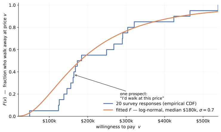
A step function built from 20 fake survey responses, with a smooth fitted over it. The point to see: is a picture of data before it is ever differentiated. Each step is one prospect saying "I'd walk at this price."
For a gentle, engineer-friendly entry to all of this, the anchor recommendation is Roughgarden, Twenty Lectures on Algorithmic Game Theory, Lectures 2–3.
Checkpoint
You can now read any pricing claim in this post as a statement about one curve fitted from data.
Part III — Virtual value, derived
What one lever move actually costs you
We'll build the machinery in three moves. First a baby example you can do with high-school calculus. Then the same three moves with a general . Then one new object — the hazard rate — with a picture.
III.1 — The complete baby example
Assume values are spread uniformly between and : everyone's willingness to pay (WTP) is equally likely to be anywhere in that range. Then
Revenue is price times the fraction who buy. The trick that keeps this at Level 1: expand the product into a polynomial so we never need the product rule.
Differentiate term by term — no product rule, nothing skipped:
Set it to zero:
Now add a marginal cost . Profit is per sale times the fraction who buy. Expand again:
There's a second route that needs no calculus at all. Demand is a straight line from down to full participation at price zero; revenue is the area of the rectangle tucked under that line whose upper corner sits at your chosen price. That rectangle is largest when the corner sits at the midpoint of the demand line — again . Two independent routes to the same answer is the strongest reassurance a Level-1 reader can get.
You just did the entire theory. Everything from here is the same three moves — write revenue, differentiate, set to zero — with a general in place of a straight line.
III.2 — The general derivation
Drop the straight-line assumption. Revenue for any distribution is
Differentiating needs the product rule this time. The fast-lane result:
Slow lane — the product rule, every step
Write as a product with and . The product rule is . Here and (the derivative of is ). So
Now the one clean move that produces the hero of this post. At the revenue peak ; divide through by — a density, so it's positive and dividing is safe — and rearrange:
The left-hand side earns a name. Define the virtual value:
(The auction-theory literature — including Roughgarden and the Brown AGT notes — usually writes this as ; it's the same object.)
Read it as a bias-corrected value: the naive value , minus a tax you pay on account of everyone whose value sits above . Revenue climbs as you cut price exactly while is still negative, and peaks where crosses zero. In Part IV, cost will do something very small: it will raise that crossing from to .
A sign worth respecting — why not just write R′ = f·ψ?
If you factor out of the fast-lane result you get — note the minus. It's direction-of-travel: measures revenue per extra unit sold, and raising price sells fewer units, so in price-space the sign flips. Work in quantity instead and the minus disappears entirely: , exactly. That is the honest one-line definition — virtual value is marginal revenue, per unit sold — the reading that Bulow & Roberts (1989), The Simple Economics of Optimal Auctions, build the whole theory on.
Check it on the uniform case: — precisely the from III.1. ✓
Uniform thread ✓ #1
For Uniform we have and , so , giving
We'll set in Part IV and recover the baby example exactly.
III.3 — The hazard rate
The correction term is worth its own object. Its reciprocal is the hazard rate:
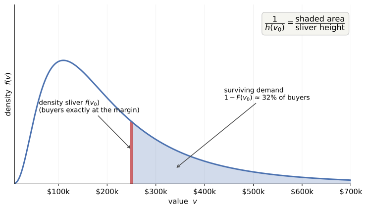
The surviving demand — the buyers above the point — is shaded; the density sliver sits right at . Then is "shaded area per unit of sliver": how many buyers still remain, per buyer sitting exactly at the margin.
A bridge for anyone who's done reliability engineering. This is the exact same hazard rate as in failure analysis — just replace "time to failure" with "willingness to pay." A constant hazard rate is the memoryless exponential distribution, the way constant-failure-rate components have exponential lifetimes.
What it means for pricing. A fat tail (lots of high-value buyers far out to the right) means a small , which means a big correction , which pushes far below the raw value . Fat tails are where naive pricing goes most wrong.
Uniform thread ✓ #2
For Uniform, . The correction shrinks to zero as : the correction vanishes for the highest-value buyer. Keep that in your pocket — it quietly foreshadows "efficiency at the top."
Checkpoint
You can now compute for any you can differentiate — and say in one sentence what it measures.
Part IV — Where cost enters
Cost sets the intersection, not the price
Cost has been waiting in the wings. Watch how little it does.
IV.1 — The one-line solve
Profit for a general is
Same two moves as III.2 — the product rule (now with , still ), then divide by :
which is one line:
That's the whole post. Demand fixes the entire shape of ; cost is a single horizontal line; the optimal price is where they cross.
Uniform thread ✓ #3
For the uniform case, , so becomes , i.e. — the same answer as III.1, now derived the grown-up way.
IV.2 — Sanity checks
An engineer will poke the edges, so let's beat them to it.
- : the price does not go to zero. In the uniform case , not . Pricing is not cost recovery — even a free-to-produce product has an optimal price set entirely by demand.
- Point-mass (all buyers at one value ): argue directly. If everyone
values it at exactly , charge ; cost only decides whether to sell at
all. So whenever .
Footnote — the formula is undefined here, and that's fine
At a point mass, is a Dirac delta, so is a -ish object and is formally undefined. Take a narrow-uniform limit around and , agreeing with the direct argument. The formula doesn't contradict the edge case; it just declines to be evaluated exactly on it.
- Non-monotone : if isn't increasing, the crossing may not be the whole story. One sentence for now; the Appendix pays it off.
IV.3 — Four distributions
Every row below is re-derivable by hand with the III.2 recipe.
| Support | Pass-through | ||||
|---|---|---|---|---|---|
| Uniform | |||||
| Exponential | |||||
| Pareto | |||||
| Log-normal | no closed form | numerical | numerical | between |
For the closed-form rows, and are explicit — for the exponential and for the Pareto — so the table is an exercise set with answers, not an appeal to authority.
The last column is the pass-through rate: the fraction of a $1 cost increase that lands on the price. It runs / / across the rows.
Why can pass-through exceed 1 — why raise price by more than a dollar when cost goes up a dollar? Because of the fat tail. Raising price on a Pareto population sheds proportionally few buyers (the ones who remain are far out in the tail and barely flinch), so the optimal response to a cost shock is to retreat further up the tail and serve fewer, richer buyers. That's luxury-market behavior — and here it's derived, not asserted.
IV.4 — The pass-through theorem
How does the optimal price move when cost moves? Differentiate . Fast lane:
Slow lane — implicit differentiation, written out
The optimal price is a function of cost, ; it obeys for every . Differentiate both sides with respect to . The right side gives . The left side needs the chain rule — depends on only through — so
No-calculus verification
Two table rows become unit tests of the theorem.
- Uniform: , so the slope in is by inspection. And , giving ✓.
- Exponential: , slope by inspection. And , giving ✓.
The theorem also tells you when pass-through exceeds 1: whenever , i.e. when is flat — exactly the fat-tail regime.
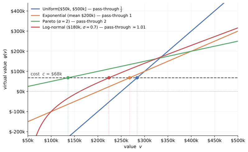
for uniform, exponential, Pareto (), and log-normal on one axis; the horizontal cost line at ($68k); the four intersections are the four optimal prices, with pass-through rates (, , , ) in the legend. This is the money figure: one equation, four demand shapes, four prices. A bonus worth noticing: the log-normal's pass-through at its optimum computes to — at this operating point it behaves almost exactly like the exponential.
IV.5 — Code
Numeric plus a root-find works for any , including the log-normal that has no closed form — same three lines.
import numpy as np
from scipy.stats import lognorm
from scipy.optimize import brentq

def psi(v, F, f):
    return v - (1 - F(v)) / f(v)

# Example: log-normal WTP, median $180k, sigma = 0.7
s, scale = 0.7, 180_000
F = lambda v: lognorm.cdf(v, s, scale=scale)
f = lambda v: lognorm.pdf(v, s, scale=scale)

c = 68_000
p_star = brentq(lambda p: psi(p, F, f) - c, 1.0, 5_000_000)
print(f"optimal price ≈ ${p_star:,.0f}")
Run this on your own WTP survey data Monday morning. (We'll use exactly this snippet — and its output — in Part VI.)
IV.6 — Decoder ring: the Lerner index
You now own the result from every seat at the table, so here is the economist's dialect for it.
If you ever talk to an economist
The condition is, in their dialect, the Lerner index:
Elasticity is just the hazard rate in disguise. Same equation, three vocabularies. Now you speak their language.
The same object, seen from three seats at the table:
| Perspective | Object | Formula |
|---|---|---|
| Buyer side | Virtual value | |
| Seller side | Marginal revenue per extra unit sold | |
| Economist's dialect | Lerner index |
IV.7 — The auction reframing
Here's the one auction line we promised. Myerson's rule (Myerson, 1981): allocate to the bidder with the highest , provided , else don't sell. In an auction, cost is a reserve price; in posted pricing, it's a floor. Same math, same role — and it closes the loop on Part II: this is literally what the FCC's economists were computing. Their reserve price is your cost line; their bidders' virtual values are your . Roughgarden's Lecture 3 is the gentler entry.
Checkpoint
You can now derive the optimal price for any you can write down — and predict how it moves when cost moves.
Part V — Where competitors enter
Competitors are demand, not strategy
A competitor changes what a buyer's alternative is worth, and that's all. Let a buyer's best outside option be (the utility of the competitor's product minus its price). The buyer's net value for you is . Refit the distribution on instead of — call it — and the pricing equation is untouched:
The equation is the interface; competitors, costs, and demand estimates are implementations behind it. Separation of concerns, in a pricing model.
Uniform thread ✓ #4 (assumption stated)
Suppose every buyer's best alternative is that one competitor. Then a $100 competitor price cut shifts the whole support of down by $100, and by the pass-through rate , your optimal price falls by exactly $50. Arithmetic, no calculus.
If only some buyers face that competitor, becomes a mixture of shifted and unshifted populations — and mixtures are exactly where can go non-monotone. That's the second time this post has pointed at the Appendix; mixtures are where the ironing machinery earns its keep.
Notice that nothing new happened mathematically in this whole section. That's the point — a deliberate breather after the IV.4 spike. The profundity here is conceptual, not technical.
One aside for completeness: genuine strategic competition (Bertrand, Cournot) shows up when competitors react to you. This post lives in the world where competitor prices are exogenous inputs to .
When this is the wrong model
Three honest boundaries. (1) Best response, not equilibrium. gives your optimal price given competitors' prices; a market equilibrium is every firm solving its own copy at once — a fixed point this one-shot tool doesn't find. (2) The perfect-substitute limit. As differentiation vanishes, collapses to a point mass at "competitor's price plus your quality edge," and the point-mass check from IV.2 says charge exactly that — match-and-undercut, whose fixed point is the Bertrand race with margins pinned to differentiation value. The equation computes every round correctly; it just doesn't tell you the spiral exists. (3) It's static. It maximizes this period's profit per customer, so growth-motivated underpricing — land-and-expand, network effects, lifetime value over first-year revenue — is deliberately out of scope. These caveats bite hardest for fast, horizontal SaaS; the procurement-sticky, few-rival gov-tech example in Part VI sits near the model's sweet spot, where residual demand market demand.
Checkpoint
You can now turn a competitor's price move into a predicted move of your own optimal price — with arithmetic.
Part VI — Case study: pricing an AI document-review SaaS
Doing this for real
Pre-publication note
These numbers are a genericized stand-in for a hypothetical "AI
document-review SaaS." Scale or reframe before publishing — the pedagogy
survives; the negotiating leverage shouldn't leak. If you rescale, the
figures are linked: the $95k/$284k/$190k base case and the $115k–$214k
sweep range appear in VI.5 and Part VII; the $224k / $284k /
$343k trio appears in VI.6 and Figure 4. Move
each set together, or re-run generate_figures.py, which wraps the IV.5
snippet and recomputes every figure and headline number from the parameters
at the top of the file.
VI.1 — Anchoring WTP
A permit review that a human does in hours at wage , which our tool automates at capture rate , is worth roughly
where the second term is the delay side: is the fraction of permits where faster review actually avoids a delay, the days saved, and the applicant's cost per day of delay. With , , and around $60/hr, the labour term alone anchors about $240 per permit. Total engineering value scales with volume: .
One honest wedge before the bands below: a public-sector buyer does not pay engineering value dollar-for-dollar. Budget caps, procurement friction, and status-quo bias take a haircut, so realized willingness-to-pay is a fraction of . (Multiply it out for a mid city — dollars of modeled value against a WTP band topping out at $500k — and you can see the haircut. Treat the $240/permit as an upper anchor, and the bands as what survives procurement.)
VI.2 — Segments
| Segment | Permits / yr | Annual WTP band |
|---|---|---|
| Small city | ~1,000 | $50k – $150k |
| Mid city | ~8,000 | $50k – $500k |
| Large city | ~30,000 | $300k – $2M |
VI.3 — Cost model
For a mid-city deployment at , that's — about $68k per year.
VI.4 — Worked example
Take the mid segment and model value as (in dollars), with cost .
Uniform thread ✓ bonus — the lower endpoint drops out
For Uniform, and , so the correction is — the lower endpoint cancels entirely. Hence exactly as before, and gives , valid whenever that lands above .
Participation is . The margin on a customer you win is ($216k); weighting by the 48% chance that a given prospect buys at this price, the expected profit per prospect is about $104k.
VI.5 — Cost-sensitivity sweep
| Naive "cost + 40%" | Δ vs naive | ||
|---|---|---|---|
| $40k | $270k | $56k | $214k |
| $68k | $284k | $95k | $189k |
| $100k | $300k | $140k | $160k |
| $150k | $325k | $210k | $115k |
At the base case (cost $68k), cost-plus charges $95k against the optimal $284k — about $190k left on the table, a 3× underprice. That surplus doesn't vanish — it goes to customers, not because they earned it, but because the seller measured the wrong quantity. This is the figure the TL;DR promised to compute — and there it is. The effect only sharpens as the product gets cheaper to run: the gap widens toward $214k (a 5× underprice) at low cost and narrows to $115k (1.5×) at high cost — because naive cost-plus tracks cost while the optimal price barely moves. (That last part is the pass-through theorem in action: each $1 of cost shifts by only $0.50, since .)
VI.6 — How wrong can your F be?
Here's the question every engineer has been holding since Part II: comes from a survey — how much does care if I fitted the wrong curve? Answer it by comparison, using the IV.5 code on the same survey data:
- Uniform fit over (dollars) → = $284k.
- Log-normal fit, median $180k, → ≈ $224k.
- Log-normal fit, median $180k, (heavier tail) → ≈ $343k.
Three defensible fits of one survey span roughly $224k–$343k — a ±21% band around the uniform answer. That band is your model-uncertainty error bar, and notice it is wider than the entire cost-sensitivity sweep above: for this product, fitting carefully matters more than measuring precisely. The direction of the error depends on where the fit puts its mass — a median-$180k log-normal concentrates buyers lower than the uniform (price drops), while fattening its tail to pushes the optimum up past both. The pass-through machinery is doing double duty here: it's also your error-propagation tool. A steep means is insensitive both to a mis-estimated cost and to a mis-fitted tail.
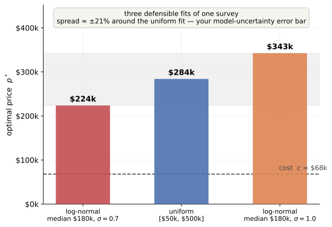
Three fits of the same survey, three optimal prices: log-normal ($224k), uniform ($284k), log-normal ($343k). The shaded band across the bars is the model-uncertainty error bar. All three numbers are computed, not typed — generate_figures.py wraps the IV.5 snippet.
One honesty note: stated preference overstates WTP — surveys are optimistic. Treat a survey-fitted as an upper anchor and update from real win/loss data. (A full treatment of that is another post.)
VI.7 — Menu design teaser
Why three tiers? A menu lets buyers sort themselves — the same virtual-value machinery applied to types rather than prices. Tier-price ratios come from virtual-type ratios, not cost ratios. That's Part 2. (Mussa–Rosen, 1978.)
Checkpoint
You can now run this entire pipeline — WTP anchor → fit → solve → stress-test the fit — on your own product.
Part VII — The meeting, revisited
Back to the whiteboard from Part I. Each strategy now gets its verdict, in the machinery's own words.
- Cost-plus measures the wrong quantity. Cost enters the problem exactly once — as the height of a horizontal line — and in our sweep, pricing off it instead of off demand left $115k–$214k per customer per year on the table.
- Match the competitor confuses an input with a strategy. A competitor's price is a term inside ; when they cut $100, your optimal response was a computable $50 — the pass-through rate — not imitation.
- Charge what it's worth had the right instinct and the wrong object. "Worth" is a distribution, not a number, and the chargeable point inside it is wherever crosses .
Which is to say: three take-home theorems, each stated twice — symbols, then meeting-ready words.
- Pricing. — "Demand fixes the curve; cost picks the intersection."
- Pass-through. — "How much of a cost shock reaches customers depends only on the slope of ."
- Competitor neutrality. — "Competitors change the distribution, never the equation."
One equation — — and everything else (cost, competitors, distribution shape) enters through its two sides.
Auctions & Mechanism Design
This post asks how a seller should set one price to maximize revenue when buyers' values are hidden. Its sibling, VCG Auctions, Gently: Pay for the Harm You Cause, asks how to allocate multiple goods efficiently while making truth-telling a dominant strategy.
Appendix — for the very curious
Nothing below is needed for anything above. Two threads planted earlier (the non-monotone in the IV.2 sanity checks, the mixture caveat in Part V) get paid off here.
A.1 — Regularity and ironing
can be non-monotone when has bumps — precisely the segment mixtures of Part V. The fix is ironing: replace with its concave envelope over the offending region. Practically, some buyer types end up pooled at one price. See Myerson (1981), §5, or Hartline's Mechanism Design and Approximation (free draft, CS-friendly), chapter 3.
A.2 — Multi-dimensional types
When a buyer's type has two dimensions at once — say volume and per-document value — the problem gets genuinely hard (Rochet–Choné, 1998). For our document-review example the two dimensions correlate strongly, so a one-dimensional type index usually suffices.
Reading list
- Brown CSCI 1440/2440 (Algorithmic Game Theory) — where I first met this machinery; its Myerson lecture derives the same (there ) through the incentive-constraints route.
- Bulow & Roberts (1989), "The Simple Economics of Optimal Auctions" — the marginal-revenue derivation this post follows, and the natural bridge for readers arriving from an AGT background.
- Roughgarden, Twenty Lectures on Algorithmic Game Theory, Lec. 2–5 — anchor.
- Myerson (1981), "Optimal Auction Design."
- Hartline, Mechanism Design and Approximation — free draft; ironing.
- Wikipedia: Vickrey auction, failure rate, Lerner index, price elasticity, Bertrand, Cournot.
- Mussa–Rosen (1978) — the Part 2 menu-design teaser.